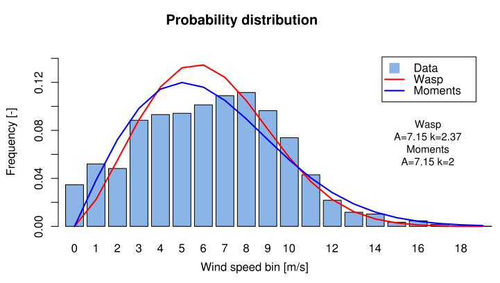
The wind speed distribution is significant for wind turbine design because it determines the frequency of occurrence of individual load conditions. The wind speed distribution is a synthetic way to describe the wind speed characteristics of a site.
A wind speed bin identify a range of wind speeds which probability of occurrence have a certain value. For example if a bin is 1 m/s wide, the wind speed bin of 5 m/s expresses the probability of the wind speed U to be 4.5 m/s ? U < 5.5 m/s.
Calculation of Weibull distribution coefficients, from wind speed measurements
The wind speed distribution is normally approximated with a Weibull distribution. Here I describe three different methods to estimate the coefficients (the scale factor A and the shape factor k) of the cumulative Weibull distribution function (equation 4.6).

The methods can be compared in several conditions but there is not a method which is the best overall. When using the Weibull coefficients to estimate the extreme wind is important a good match at the high wind speed bins. When using the Weibull coefficients to estimate the annual energy production of a wind turbine, the best method is the one that results in a predicted energy production closer to the one calculated directly from the measured distribution. In this case it is therefore important a good fitting for the wind speed bins that corresponds to the slope of the wind turbine power curve.

Method 1: 1st and 2nd moments
The method uses two parameters calculated from the data set:
- The average wind speed, which is the first moment

- The variance of the mean wind speed, which is the second moment ?2.
These two numbers can be calculated from the Weibull coefficients through equation 4.7 and
4.8.
The first moment:

(4.7)
The second central moment:

(4.8)
By squaring the first equation and dividing by the second, an equation in k is obtained(equation 4.9). Solving equation 4.9 with a zero-finding function can return k. Then, A is calculated from equation 4.7.

(4.9)
Method 2: WAsP method
The method uses three parameters calculated from the data set:
- the average wind speed, which is the first moment (eq 4.7),
- the average of the cubed wind speed measures, which is the third moment (eq 4.10)
- the value of the cumulative wind speed distribution Fµ for which the wind speed is lower than the average wind speed.
The third moment:
![]()
(4.10)
By combining the equations 4.6 and 4.10, an equation with only k unknown is obtained (equation 4.11). Solving that equation with a zero-finding algorithm will return k. Then, A is calculated from equation 4.7.

(4.11)
Method 3: Log-log method
The method uses the values of the probability distribution of the wind speed (F), hence a value for every wind speed bin. By plotting a graph with equations:

(4.12)
an almost straight line should be obtained. Then by fitting a straight line with a least-squared method (for example the “lm” function of R) the slope of the line (m), the intersect to the ordinate axis (y0) allows to calculate the Weibull coefficients as:

(4.13)
Note that when the wind speed distribution described by Weibull coefficients is used to calculate energy production, since the wind turbine is not working for wind speed lower than cut-in and higher than cut-out, those wind speed bins can be discarded in the fitting process.
Also, at wind speed between rated wind speed and cut-out is not very important to have good fitting because the wind turbine will be at full power output anyway. A good improvement of this method would be to use a fitting algorithm that weight the error using the specific power curve, optimizing for the minimum.
Implementation notes
That “L upside down”
is called the “lambda function”. It is actually a function which you find in the program you use to calculate the equations. What is inside the bracket soon after the lambda is the argument of the function, not a multiplication!
“My umulative weibull distribution is more than one, like1,98”
The sum of the probabilities of a probability distribution should be equal to one. On your wind speed date you might have missing measurements, and your sum will be lower than one. It is ok.
Bins of 1m/s or 0.5 ms. If you calculate the cumulative probability of your probability distribution made with bins of 0.5 m/s your sum will end up a bit less than 2. This is because a cumulative sum is like integrating, which is like calculating areas. If you want the area of one of those vertical blue bars of the figure on top of this page you have to sum the heights multiplied by the width, which is 0.5 m/s (or 1m/s). If you do this your maximum cumulative value will be correct, and a bit less than 1.